Computing years of lost life: why actuaries really need to be able to do counterfactual reasoning

Hugh Osmond recently put out this interesting twitter thread:

 

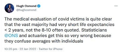
Although the average age of death in the UK is around 82, if a person reaches 82 then on average (i.e. without knowing any details of the particular person) the person can expect to live about another 8 years. We know the average age of a person dying from Covid is also 82, so it seems reasonable to assume that a typical person dying from Covid loses 8 life years. But, as Hugh points out, this reasoning is flawed. Hugh provides what is essentially an informal argument. In what follows we provide a formal explanation.

The question we are trying to answer is:

Knowing that an individual (let’s say it’s a man called Fred) has died from Covid at the age of 82, how much longer would Fred have lived if he had not got Covid?

This is a classic ‘counterfactual’ question. We want to know what would happen to Fred in an alternative world if something that happened in the real world (namely, getting Covid) was changed. And we want to take account of everything we can learn about Fred that will be unchanged in the counterfactual world from what happened in the real world. 

Crucially, because we know that Fred died of Covid, we learn from the real world that (compared to the average 82 year-old) Fred is much more likely to also have had some critical pre-existing illness. And this knowledge must be retained in the counterfactual world.

As very well explained by Judea Pearl, answering counterfactual questions requires a causal model and an inference method that are beyond what can be achieved with traditional statistical methods.  In what follows we use illustrative and simplified assumptions to explain this counterfactual reasoning.

First, we need a causal model of the ‘real world’. Such a basic causal model is shown in Figure 1.

 

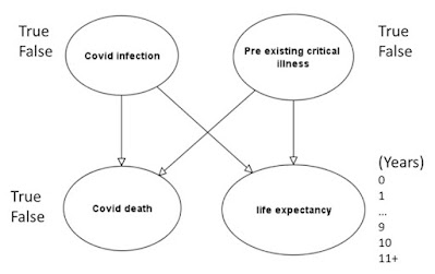
Figure 1 Basic causal model (for 82 year-olds)

This tells us that whether a person suffers a Covid death depends not just on whether the person becomes infected, but also on many other factors including whether the person has a pre-existing critical illness. Similarly, a person’s life expectancy depends on the same factors (among others).

When we assign prior probabilities to the nodes ‘Covid infection’ and ‘Pre-existing critical illness’, and conditional probabilities to the nodes ‘Covid death’ and ‘life expectancy’, then the causal model becomes a Bayesian network for which we can perform Bayesian inference.

In what follows we use the following assumed prior and conditional probabilities:

•  Covid infection: 1%
•  Pre-existing critical illness: 10%
• Covid death given Covid infection is false = 0%
•  Covid death given Covid infection and Pre-existing critical illness = 10% 
•   Covid death given Covid infection and no Pre-existing critical illness = 0.1%
• The full set of conditional probabilities for life expectancy is given in Table 1

Table 1 Conditional probability table for 'life expectancy'

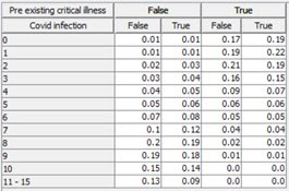
Changing any of these probability assumptions (within reason) does not change the thrust of the argument (readers are free to try out the model and make their own changes using their favourite Bayesian network software**).

With these assumptions we get the prior marginal probabilities shown in Figure 2.

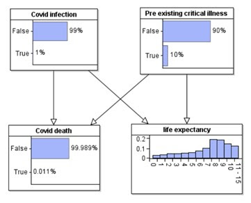
Figure 2 Prior marginal probabilities

So, in the real world the median life expectancy of an average 82-year-old is 8 years.  

But, if we know that an individual dies from Covid then, while obviously this means that ‘Covid infection’ must be true,  through Bayesian inference we also get the revised probability for ‘pre-existing critical illness’ shown in Figures 3.  

 

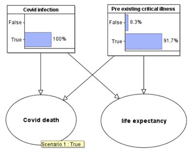
Figure 3 Revised probabilities are observing Covid death

We can now use this new information about the probability this individual has pre-existing critical illness in a counterfactual world where he is not infected with Covid. The counterfactual model required for this is shown in Figure 4.

 

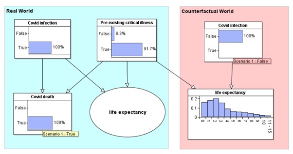
Figure 4 Counterfactual world

The ‘Covid infection’ and ‘life expectancy’ nodes in the counterfactual world are simply copies of the same named nodes from the real world model. They have exactly the same prior and conditional probability tables respectively. When we enter ‘Covid infection’ is false in the counterfactual world, we get the revised probability distribution for life expectancy. This individual has a median of 2 years life expectancy, rather than the 8 years.

The inference performed in this counterfactual model is not possible using the original model alone.

For more information on Bayesian networks and counterfactual reasoning see our book and short videos.

 **The model used here can be downloaded and run in the free trial version of AgenaRisk (we declare an interest - Directors of the company that owns the software).

 29 Jan update:  Here is a 5 minute video explanation on the above with an even simpler model (that can be downloaded by right clicking)

 

 

Claim that "1 in 3 people who have the virus have no symptoms" is a misleading exaggeration

 

28 Feb 2021  DRAFT ONLY: This article is under review and will be updated. An updated analysis with new data from the Cambridge study is here

One of the major messages currently being pushed everywhere by the UK Government about COVID-19 is the claim that "1 in 3 people who have the virus have no symptoms". 

A person is classified as having COVID if they get a positive test result and it has long been conjectured that (for PCR tests) many of these are false positives especially for people who have no symptoms and where there was no confirmatory test (the new evidence below provides further confirmation of this). So, clearly, it is possible that a large proportion of people classified as having the virus (as opposed to actually having the virus) have no symptoms. But, the new evidence suggests that either the "1 in 3" proportion is massively exaggerated, or the 'case' numbers are massively exaggerated. Or (likely) a combination of both. They certainly cannot both be true. In fact, if we accept that the Government case numbers really are people who have the virus then (based on the new evidence) it turns out that between 1 in 56 and 1 in 13 people who have the virus have no symptoms - very different from the Government "1 in 3" claim. Conversely, if the "1 in 3 claim" was really correct, than it turns out that the proportion of people with the virus during 1-7 Feb was not 1.25%, i.e. 1 in 80 as claimed, but between 0.09% and and 0.29% (i.e. between  1 in 1,111 and 1 in 345).

To understand what it going on here, it is important first to note that many people who see a statement like 

"1 in 3 people who have the virus have no symptoms" 

assume this is the same as:

"1 in 3 people who have no symptoms have the virus". 

That is, in fact, a classic  probability fallacy called the fallacy of the transposed conditional (or prosecutor's fallacy) whereby the probability of a hypothesis H given some evidence E is assumed to be equal to the probability of  the evidence E given  the hypothesis H. It is not. Just think of the example where an animal is hidden behind a screen. Let H be the hypothesis that the animal is a cow. We know that almost every cow has 4 legs (we allow for a few who have lost legs). So if I give you the evidence E that the cow has 4 legs then the probability of the evidence E given H is 1 (or very close to it). But the probability of H given E (i.e. the probability the animal is a cow given that the animal has 4 legs) is certaintly not close to 1 since most 4-legged animals are not cows. 

Perhaps the Government "1 in 3" message was phrased in the way it was to deliberately exploit this very common misunderstanding.  Obviously, it is not the case that "1 in 3 people who have no symptoms have the virus", because even if as few as a half the UK population does NOT currently have COVID-symptoms, then there would be over 11 million people who have the virus but no symptoms. This is clearly wrong, since the ONS estimate for total active cases for the week ending 6 Feb is that less than one million people (1.25% of the population) have the virus (in any case, as we explain below, we believe the 1.25% is too high anyway because of the inclusion of false positives).

The new evidence that suggests that both the case numbers, and the claim that "1 in 3 people who have the virus have no symptoms", are exaggerated comes from an ongoing study at Cambridge University. This study tests students without symptoms and, for the week of 1-7 Feb, they reported that a total of 4058 students with no symptoms were tested. None of these students were confirmed as positive, although critically (as we discuss below) there were a significant number of false positives.

Here is a screenshot of the summary results:

Can we conclude that the true percentage of asymptomatic people with the virus (in the week 1-7 Feb) is 0%.  No, because this is only one sample from a large population. If we use all the recent Cambridge data (6 cases from 11,573 people with no symptoms) then we could assume that about 0.052% of people with no symptoms have the virus. However, that data was for different weeks and it is not clear how many of the same students were tested. Fortunately, there is another relevant publicly available dataset for the week of 1-7 Feb that we can use - the data on Premiership football players and staff  where we find that only 2 out of 2970 tested positive. Unlike the Cambridge study we cannot be certain that all of the 2970 players and staff tested during the week of 1-7 Feb had no symptoms. Given that footballers are among the few in the population not subject to social distancing it could be argued that (except for people in care homes and hospitals) we ought to see a higher infection rate among them compared to most of the population. If the ONS estimate of 1.25% of the population having the virus during the week of 1-7 Feb were accurate then we might expect to have found 37 cases rather than 2.  It is conservative to assume that most of the 2970 did not have symptoms. We do not know if either of the 2 positive cases had symptoms. If they did  then (together with the Cambridge study) we could conclude that, of over 7000 people with no symptoms not a single one tested positive. So, let us conservatively assume that the 2 positive cases did not have symptoms. Then, combining the Cambridge and Premier League data we have 2 ‘cases’ from 7,028 people with no symptoms, i.e. 0.0285% of those with no symptoms has the virus.

The two samples are, of course, not representative of the population. However, this sample bias should surely favour the Government claim, because if any group are really likely to have COVID-19 but no symptoms it is surely young and fit people.   

What these two samples provide is an estimate of the probability a person has the virus given that they have no symptoms. Using the Government claim of 1.25% probability a person has the virus we can use Bayes Theorem to provide an estimate of the probability a person has no symptoms if they have the virus - which the Government claims is 33% (that's the "1 in 3 claim"). The (Bayesian) 95% confidence interval estimates this probability to be between 1.8% and 7.8% with a mean value of 4.7%. So, instead of 1 in 3 as claimed the figure is between 1 in 56 and 1 in 13, with 'expected value' 1 in 21.

On the other hand if we use the Government "1 in 3" claim, we can also uses Bayes Theorem to estimate the probability a person has the virus. The (Bayesian) 95% confidence interval estimates this probability to be between 0.09% and 0.29% with a mean value of 0.2%, which would suggest the claimed 1.25% infection rate is exaggerated by a factor of over 6.

The critical additional information in the Cambridge report is the evidence it provides about false positive tests for people without symptoms as seen in this screenshot:

Critically, the study does pooled testing and then confirmatory testing on each individual case if a pooled test is positive. In the study there were 1752 pooled samples of which 13 were false positives (in the sense that when individual confirmatory testing was done on these, every sample in all 13 pooled samples was negative).  So, even in the highly skilled testing environment at Cambridge, the false positive rate (without confirmatory testing) for people without symptoms during the week of 1-7 Feb is 0.7%. This is a much higher rate than the 1 in 400 (0.025%) reported 'to date', but it should be noted that the 1 in 400 rate was also reported for the previous week so it clearly does not take account of the large number of false positives during 1-7 Feb. It is also not clear if the 1 in 400 rate includes confirmatory testing.

The Government 'case' numbers are based on mass PCR testing and there is no evidence that any confirmatory testing has been undertaken as previously reported on this blog. The mass PCR testing will certainly have a higher false positive rate for people with no symptoms than that at Cambridge.  This is very important for understanding why the Government 'case' numbers - as well as the "1 in 3" claim are exaggerated. Based on the Cambridge data and some other reasonable assumptions it follows that a high percentage of those without symptoms testing positive are false positives (the report will provide the full Bayesian analysis).

 

See also:  

NFL: All 77 NFL positive covid-19 tests were false positives

Lions' Matthew Stafford glad false-positive led to covid-19 testing change

 All COVID-19 articles on this blog

What can we learn from very few data points (with implications for excess death numbers)?

Let's suppose that a museum decides to spend money in Sept 2020 advertising for new members. To see if the advert has worked you manage to find the data for numbers of new members (adjusted for changing population size) in October in each of the 5 previous years. The numbers are:

• Oct 2015: 176
• Oct 2016: 195
• Oct 2017: 169
• Oct 2018: 178
• Oct 2019: 162

Suppose that, in Oct 2020, we see 178 new members. This is above the preceding 5-year average of 176, but we actually saw higher numbers in two of the five previous years. So, nobody would seriously suggest that the 'above average' number of new members was due to the advertising. But what if we saw 197 new members? Or 200, 210, 220, 250?  At what point could we reasonably conclude that the number is sufficiently 'higher' for there to have to be some causal explanation such as the advertising or some other factor?

The classical statistical aproach to answering this question is to 'fit' the data to a statistical distribution, such as a Poisson or Normal distribution. This enables us to determine the range within which we would 'expect' a new number to fall if there had been no intervention. The Poisson distribution 'fit' for the 5 years is:

Note: the Poisson distribution has just one parameter, namely the mean which is 176 in this case; the variance is the same as the mean

So, if we set the threshold at 95%, and observed say 200 new members, we might conclude - as evidence to support the impact of the advertising - that:

"The number of new members significantly exceeds the 5-year average (95% confidence bound)."

(The best fit Normal distribution has mean 176 and variance 152.5 so is 'narrower' than the Poisson above, with slightly lower percentiles, namely 196 and 204 for the 9% and 99% respectively, so if we felt that was a more reasonable model, we would conclude that a value of 197 was above the 95% confidence bound for the 5-year average).

But, even with the tiny sample of 5 data points we have one datapoint of 195 (in Oct 2016) which is very close to being beyond the 5-year upper 95% confidence bound. So why should we consider 200 especially high? 

Indeed, if we had data for more than 5 previous years of October new members, we might discover that every 10 years or so there is an October surge due to things that have nothing to do with advertising; maybe, there are major school initiatives every so often, or a local TV station runs a story about the museum etc. Perhaps in Oct 1998 there were 2000 new members in October which is assumed to have been due to a Hollywood movie having a set filmed there then. So, assuming it was available and adjusted for population size, how far back should we go with the data?

If we really must rely on such tiny datasets for making the kind of inferences here, then simply 'fitting' the tiny dataset to a particular distribution does not capture the full uncertainty we have about new member numbers. Fortunately, the Bayesian approach to learning from data enables us to accommodate this type of uncertainty along with any prior knowledge we have (although in this case we do not include any explicit prior knowledge). The Bayesian model* (see below for details) produces quite different results to the standard distribution fitting models. The 95% and 99% upper confidence bounds turn out to be 205 and 227 respectively. In other words, if there were say 204 new members in October 2020 then we would not be able to reasonably claim that this exceeded the 5-year average upper 95% confidence bound. 

It is also important to note that, using just 5 data points also make the results extremely sensitive to small changes. Suppose, for example, that the 2019 was not 162 but was 120 (with all other numbers exactly the same). Then, although this makes the 5-year average much lower (it drops to 166) the (Bayesian learnt) distribution becomes 'wider' (i.e. the variance inceases) so that the 95% and 99% upper confidence bounds turn out to be much higher at 236 and 294 respectively.

You may be wondering why these differences are important. It is because the number of 'excess deaths' is now widely used as the most important indicator of the impact of  COVID and/or lockdowns. And one of the standard approaches for determining whether increased death counts are likely explained by COVID and/or lockdowns is to use the previous 5-year datasets of death numbers and the model 'fitting' approach described above.

Indeed this issue - and the limitations of using such 5-year averages - is the subject of this very interesting analysis "Home Depot, Hogwarts, and Excess Deaths at the CDC"  by Kurt Schulzke. 

In fact, the 2015-2019 numbers used in the hypothetical museum example above are exactly the week 15 numbers for fatalities per million of the population for the state of Nebraska.

Based on the CDC approach (which uses the Poisson distribution) if the week 15 number had been above 198 it would have been classified as beyond the 5-year average upper 95% confidence bound. But a number above 205 would have been required for the more realistic Bayesian approach. The actual number was 178 - which could still be reported as being 'above the 5-year average' but is, of course, not at all unusual.

So what this all means is that you need to be very wary if you see conclusions about the current week, month or year death numbers being 'significantly above the 5-year average'. 

Here are the details for those interested in the Bayesian learning models (you can run these models, including with different values using the free trial version of AgenaRisk (www.agenarisk.com); the model you need is here (right click and 'save as' to save this as a file which you then open in AgenaRisk)

 

 

*As you can see from above we considered two different Bayesian models, one based on the Normal distribution and the other based on the Poisson. The problem with the Poisson distribution is that it is most suited to those situations where we are measuring the number of occurences of fairly rare events in a given period, so that the number are typically very low (like number of buses arriving at a stop every 10 minutes). Also, its assumption of a constant mean rate equal to the variance is intrinsically contradicted by death data. Even before COVID19, different types and severity of flu at different times of the year (from one year to the next) causes significant fluctuations which, over a long period, cannot be 'fitted' well to the 'narrow' Poisson distribution. Hence, the Normal distribution - whose variance is independent of the mean and which can be 'learnt' from the data - is more suitable. However, even the Normal will generally be too 'thin tailed' to properly model unusual and rare deviations which might be expected with death data.

See: "Home Depot, Hogwarts, and Excess Deaths at the CDC"  by Kurt Schulzke.

The need for causal models to understand and explain whether statistics provide evidence of racially biased policing

Even before the recent George Floyd case, there has been much debate about the extent to which claims of systemic racism are supported by statistical evidence. Contradictory conclusions have been made about whether unarmed blacks are more likely to be shot by police than unarmed whites using the same data. The problem is that, by relying only on data of ‘police encounters’, there is the possibility that genuine bias can be hidden.

In this short paper we provide a causal Bayesian network model to explain this bias – which is called collider bias or Berkson’s paradox – and show how the different conclusions arise from the same model and data. We also show that causal Bayesian networks provide the ideal formalism for considering alternative hypotheses and explanations of bias.

Fenton N.E., Neil M, Frazier S (2020), "The role of collider bias in understanding statistics on racially biased policing", http://arxiv.org/abs/2007.08406

The Deer Hunter: A lesson in the basics of risk and probability assessment

I was recently watching a re-run of the classic 1978 Michael Cimino film “The Deer Hunter”. It contains one of the most iconic scenes in cinema history involving a ‘game’ of Russian roulette forcibly played by two American soldiers held captive in Vietnam. Although I have seen the film several times, this scene never seems to lose its impact. As I am currently teaching a new course on Risk Assessment and Decision Making, it also occurred to me that the scene provides a rich source of examples to illustrate core concepts of probability and risk including: probability and odds, basic probability axioms, conditional probability, risk and utility, absolute versus relative risk, event trees, and Bayesian networks.

So, I have written a short paper which hopefully has something of value both for people with no background in probability/statistics and also people who do, but want to find out more:

Fenton, N. E. (2020). The Deer Hunter: A lesson in the basics of risk and probability assessment. https://doi.org/10.13140/RG.2.2.31675.98089.

(The Bayesian network models described in the appendix of the paper are in this file which can be run using the trial version of AgenaRisk

 I have also made a video based on the paper, which includes the actual scene from the film with my narrative:

Simpson's paradox again: fixing an example from Pearl's "Book of Why" (with video)

I've written about Simpson's paradox before. Given its importance in highlighting the need for causal explanations of observed data, I've been using it to motivate students on my new module on risk assessment and decision analysis for data science.  I have put together a couple of videos with examples to explain it graphically (see below). I wanted to base one of the videos on the example of 'exercise v cholesterol' presented in the excellent "Book of Why" by Pearl and Mackenzie:

But it turns out there is a problem with this example. It assumes that in the 'data' in the real world (the left hand figure), older people are the ones who do most exercise. This is clearly not the case. At first I thought this was due to a simple ‘typo’ in that they labelled the age groups the wrong way round (i.e. the 10 – 20 – 30 – 40 – 50 age groups should be reversed). But if you reverse them you hit a different error – this time it would show that older people have lower cholesterol than young people, which is again clearly wrong. So whichever way you spin this, the example simply does not make sense in the ‘real world’ because it does not make sense for the chosen attributes.

However, the example can be 'fixed' by considering instead 'exercise v junk food consumption' because - in the real world - it is the case that older people not only exercise less than younger people but they also eat less junk food. (**22 March 2020 UPDATE) 

I have prepared a (6-minute) video using this example:

And here is another video (5-minutes) explaining a more common example of Simpson's paradox:

**22 March 2020 update: It seems that in some age categories there might be a problem also with my assumption. My colleague Marko Tesic points out:

I’m just wondering about the relationship between exercise and junk food intake within each age group. I’m not sure the association is negative for each age group (although I do think that when considering the whole population this association is positive). People who exercise often eat quite a lot: the more people are active the more fuel their body needs to recover, in particular if people want to gain muscle weight (which is often the case with young people). Now, it’s not unlikely that a bunch of the food that people who excise eat is actually junk food. The attached paper suggests exactly that. Namely, they find that many people, in particular young people, indulge in junk food after exercise. So I think that the association between exercise and junk food intake may not be negative within each age group. Rather, it’s perhaps positive for teenagers and young adults, close to no association for mature adults and negative for pensioners. This is still interesting as it’d be showing that the general population association does not hold in all age groups and that there’s a partial (rather than complete) reversal in the association.

Simone Dohle, Brian Wansink, and Lorena Zehnder (2014). Exercise and Food Compensation: Exploring Diet-related Beliefs and Behaviors of Regular Exercisers.Journal of Physical Activity and Health doi:http://dx.doi.org/10.1123/jpah.2013-0383

See also:

• Simpson's paradox again
• The Book of Why

Understanding Bayes theorem

As part of my presentation at the Wolfson Institute of Preventative Medicine today I got some audience participation using the mentimeter tool. One of the things I did was to test the participants' understanding of Bayes before and after the seminar. I posed this question*:

The results were very interesting. Before the seminar the 'average' probability answer was 76% (but note the variation in the distribution)

After, the average was  9.4%

The correct answer is just below 0.5%:

*Based on example from:  Neapolitan, Richard, Xia Jiang, Daniela P. Ladner, and Bruce Kaplan. 2016. “A Primer on Bayesian Decision Analysis With an Application to a Kidney Transplant Decision.” Transplantation 100 (3): 489–96.

Simpson's paradox again

Deepai.org have a post about our paper on Simpson's paradox (we wrote this in 2015 but only just uploaded it to arxiv). The full paper is here.

The paradox is covered extensively in both “The Book of Why" by Pearl and Mackenzie (see my review) and also David Spiegelhalter’s “The Art of Statistics: How to Learn from Data”(see my review). Speigelhalter's book contains a particularly good example of Cambridge University admissions data:

Overall the acceptance rate was higher for men and than women, but in each subject the rate was higher for women than men. This is explained by the observation that women were more likely to apply for those subjects where the overall accepance rates were lower. In other words the relevant causal model is this one:

See also: Doctoring Data