Thursday, 2 April 2020

Coronavirus: country comparisons are pointless unless we account for these biases in testing (reprint of our article in The Conversation)

Coronavirus: country comparisons are pointless unless we account for these biases in testing
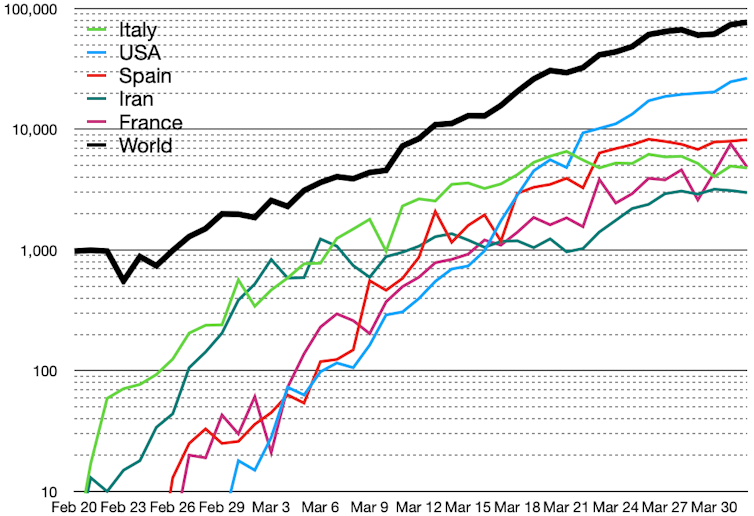

New cases daily for COVID-19 in world and top countries. Chris55 /wikipedia, CC BY-SA
Norman Fenton, Queen Mary University of London; Magda Osman, Queen Mary University of London; Martin Neil, Queen Mary University of London, and Scott McLachlan, Queen Mary University of London
 

Suppose we wanted to estimate how many car owners there are in the UK and how many of those own a Ford Fiesta, but we only have data on those people who visited Ford car showrooms in the last year. If 10% of the showroom visitors owned a Fiesta, then, because of the bias in the sample, this would certainly overestimate the proportion of Ford Fiesta owners in the country.

Estimating death rates for people with COVID-19 is currently undertaken largely along the same lines. In the UK, for example, almost all testing of COVID-19 is performed on people already hospitalised with COVID-19 symptoms. At the time of writing, there are 29,474 confirmed COVID-19 cases (analogous to car owners visiting a showroom) of whom 2,352 have died (Ford Fiesta owners who visited a showroom). But it misses out all the people with mild or no symptoms.


Read more: COVID-19 tests: how they work and what's in development


Concluding that the death rate from COVID-19 is on average 8% (2,352 out of 29,474) ignores the many people with COVID-19 who are not hospitalised and have not died (analogous to car owners who did not visit a Ford showroom and who do not own a Ford Fiesta). It is therefore equivalent to making the mistake of concluding that 10% of all car owners own a Fiesta.

There are many prominent examples of this sort of conclusion. The Oxford COVID-19 Evidence Service have undertaken a thorough statistical analysis. They acknowledge potential selection bias, and add confidence intervals showing how big the error may be for the (potentially highly misleading) proportion of deaths among confirmed COVID-19 patients.

They note various factors that can result in wide national differences – for example the UK’s 8% (mean) “death rate” is very high compared to Germany’s 0.74%. These factors include different demographics, for example the number of elderly in a population, as well as how deaths are reported. For example, in some countries everybody who dies after having been diagnosed with COVID-19 is recorded as a COVID-19 death, even if the disease was not the actual cause, while other people may die from the virus without actually having been diagnosed with COVID-19.

However, the models fail to incorporate explicit causal explanations in their modelling that might enable us to make more meaningful inferences from the available data, including data on virus testing.
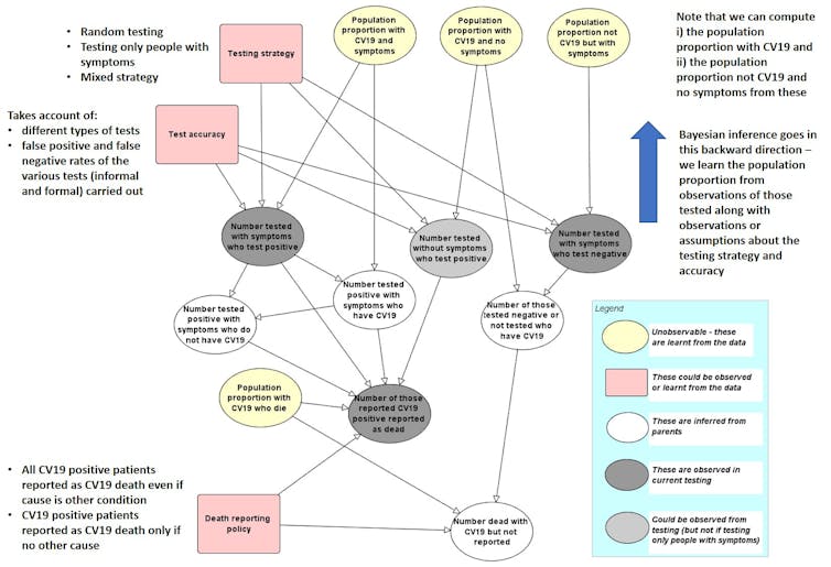
What a causal model would look like. Author provided

We have developed an initial prototype “causal model” whose structure is shown in the figure above. The links between the named variables in a model like this show how they are dependent on each other. These links, along with other unknown variables, are captured as probabilities. As data are entered for specific, known variables, all of the unknown variable probabilities are updated using a method called Bayesian inference. The model shows that the COVID-19 death rate is as much a function of sampling methods, testing and reporting, as it is determined by the underlying rate of infection in a vulnerable population.

Therefore, different countries may appear to have different death rates, but only because they have applied different sampling and reporting policies. It is not necessarily because they are managing the virus any better or that the virus has infected fewer or more people.

With a causal model that explains the process by which the data is generated, we can better account for these differences between countries. We can also more accurately learn the underlying true population infection and death rates from the observed data. Such a model could be extended to include demographic factors, as well as social distancing and other prevention policies. We have developed such models for many similar problems and are currently gathering data required for populating the kind of model that we outline in the above figure.

Random testing

In the absence of community-wide testing, only random testing applied throughout the population will enable us to learn about the number of people with COVID-19 who are asymptomatic or have already recovered. Only when we know how many people don’t show symptoms, will we know the underlying infection and death rate. It will also enable us to learn about the accuracy of the tests (false positive and false negative rates).

Random testing therefore remains the most effective strategy to avoid selection bias and reduce the distortions in reported statistics. Ideally, this should be combined with a causal model.
Random testing would be ideal. SamaraHeisz5/Shutterstock

Currently it seems there are no state-wide protocols in place in any country for randomised community testing of citizens for COVID-19. Spain did attempt it. But that involved purchasing large volumes of rapid COVID-19 tests, and they soon discovered that some Chinese-sourced tests had poor validity and reliability delivering only 30% accuracy – resulting in high numbers of false positives.

Read more: COVID-19 tests: how they work and what's in development

Countries like Norway have proposed introducing such tests, but there is uncertainty around how to legislatively compel citizens to test – and what might constitute an appropriate randomisation protocol. In Iceland, they have voluntary sampling which has covered 3% of the population, but this isn’t random. Some countries with large scale testing, like South Korea, might get closer to being random.

The reason it is so hard to achieve random testing is that you have to account for several practical and psychological factors. How does one collect samples randomly? Gathering samples from volunteers may not be sufficient as it does not prevent self-selection bias.

During the H1N1 influenza pandemic of 2009–2010, there was a lot of anxiety about the disease that created “mass psychogenic illness”. This is when hypersensitivity to particular symptoms leads to healthy people self-diagnosing as having a virus – meaning they would be highly incentivised to get tested. This could, in part, further contribute to false positive rates if the sensitivity and specificity of the tests are not fully understood.

While self-selection bias is not going to be eliminated, it could be reduced by running field tests. This could involve asking the public to volunteer samples in locations where, even in a lockdown state, they might be expected to attend and also from those in self-imposed isolation or quarantine.
In any event, it is important to note that when statistics are communicated at press conferences or in the media, it is very important that their limitations are explained and any relevance to the individual or population are properly delineated. It is this which we contend is lacking in the current crisis.


The Conversation

Norman Fenton, Professor of Risk and Information Management, Queen Mary University of London; Magda Osman, Reader in Experimental Psychology, Queen Mary University of London; Martin Neil, Professor in Computer Science and Statistics, Queen Mary University of London, and Scott McLachlan, Postdoctoral Researcher in Computer Science, Queen Mary University of London
This article is republished from The Conversation under a Creative Commons license. Read the original article.

Sunday, 29 March 2020

COVID-19: the need for more random testing combined with causal modelling

We know some strawberry flavoured sweets are contaminated. But, if wrapper colour is not a reliable indicator of the flavour of sweet it contains, what do we learn about the proportions of strawberry and contaminated sweets if we only test sweets with red wrappers?

The current COVID-19 strategic testing strategies - implemented to inform policy making - focus primarily on people already hospitalized with significant symptoms or on people most at risk. This seems to make sense for short-term medical reasons, but such testing is highly biased with sub-optimal consequences. Without understanding the causal explanations for the resulting data from such testing we end up with highly misleading conclusions about infection and death rates. Starting with an analogy of testing sweets for contamination, this short paper illuminates the need for random testing combined with causal models:
Fenton N E, Osman M, Neil M, McLachlan S, "Improving the statistics and analysis of coronavirus by avoiding bias in testing and incorporating causal explanations for the data"
2 April 2020 UPDATE: A revised and edited version of this article now appears as the lead story on The Conversation

Sunday, 15 March 2020

Simpson's paradox again: fixing an example from Pearl's "Book of Why" (with video)

I've written about Simpson's paradox before. Given its importance in highlighting the need for causal explanations of observed data, I've been using it to motivate students on my new module on risk assessment and decision analysis for data science.  I have put together a couple of videos with examples to explain it graphically (see below). I wanted to base one of the videos on the example of 'exercise v cholesterol' presented in the excellent "Book of Why" by Pearl and Mackenzie:


But it turns out there is a problem with this example. It assumes that in the 'data' in the real world (the left hand figure), older people are the ones who do most exercise. This is clearly not the case. At first I thought this was due to a simple ‘typo’ in that they labelled the age groups the wrong way round (i.e. the 10 – 20 – 30 – 40 – 50 age groups should be reversed). But if you reverse them you hit a different error – this time it would show that older people have lower cholesterol than young people, which is again clearly wrong. So whichever way you spin this, the example simply does not make sense in the ‘real world’ because it does not make sense for the chosen attributes.

However, the example can be 'fixed' by considering instead 'exercise v junk food consumption' because - in the real world - it is the case that older people not only exercise less than younger people but they also eat less junk food. (**22 March 2020 UPDATE


I have prepared a (6-minute) video using this example:


And here is another video (5-minutes) explaining a more common example of Simpson's paradox:


**22 March 2020 update: It seems that in some age categories there might be a problem also with my assumption. My colleague Marko Tesic points out:
I’m just wondering about the relationship between exercise and junk food intake within each age group. I’m not sure the association is negative for each age group (although I do think that when considering the whole population this association is positive). People who exercise often eat quite a lot: the more people are active the more fuel their body needs to recover, in particular if people want to gain muscle weight (which is often the case with young people). Now, it’s not unlikely that a bunch of the food that people who excise eat is actually junk food. The attached paper suggests exactly that. Namely, they find that many people, in particular young people, indulge in junk food after exercise. So I think that the association between exercise and junk food intake may not be negative within each age group. Rather, it’s perhaps positive for teenagers and young adults, close to no association for mature adults and negative for pensioners. This is still interesting as it’d be showing that the general population association does not hold in all age groups and that there’s a partial (rather than complete) reversal in the association.
Simone Dohle, Brian Wansink, and Lorena Zehnder (2014). Exercise and Food Compensation: Exploring Diet-related Beliefs and Behaviors of Regular Exercisers.Journal of Physical Activity and Health doi:http://dx.doi.org/10.1123/jpah.2013-0383

See also:


Friday, 13 March 2020

In the UK football was always going to be the tipping point for Coronavirus risk mitigation


Yesterday the PM announced the importance of not cancelling major sporting events; and the Premier League announced there would certainly be no cancellations of this weekend's matches. But anybody with any football knowledge knew that - whatever the Government's risk mitigation plans were for Coronovirus - they would become irrelevant if a single high profile Premiership player or manager became infected. 
As soon as it was confirmed that Arsenal manager Mikel Arteta had the virus last night, it was inevitable that a total shutdown of all professional football would start and that is precisely what has happened. Again, anybody with any UK football knowledge knows that this is also a game-changer as far as the whole UK economy is concerned. Millions who were previously unmoved to make any changes will voluntarily go into lock-down after panic buying (see the above immediate response). 
Note that nothing much changed when it was announced that the Government's own Health Minister got the virus a few days ago. But one key football person getting it was the single trigger for mass change.

I can only assume that the Government risk experts/advisors did not include a single person with football knowledge.....

p.s. from a purely selfish perspective, as a Spurs fan, I am delighted that - by the time the Premiership resumes - we might have some of these players fit again..


Friday, 17 January 2020

Understanding Bayes theorem


As part of my presentation at the Wolfson Institute of Preventative Medicine today I got some audience participation using the mentimeter tool. One of the things I did was to test the participants' understanding of Bayes before and after the seminar. I posed this question*:


The results were very interesting. Before the seminar the 'average' probability answer was 76% (but note the variation in the distribution)


After, the average was  9.4%


The correct answer is just below 0.5%:


*Based on example from:  Neapolitan, Richard, Xia Jiang, Daniela P. Ladner, and Bruce Kaplan. 2016. “A Primer on Bayesian Decision Analysis With an Application to a Kidney Transplant Decision.” Transplantation 100 (3): 489–96.

Wednesday, 11 December 2019

Problems with DNA mixed profile evidence: the case of Florencio Jose Dominguez


I have written many times before about the potential problems when using the likelihood ratio (LR) as a measure of probative value of evidence. The problems are especially acute when the evidence consists of a tiny sample of DNA for which there are at least two people contributing - often referred to as a low template mixed DNA profile. Over the last year I have been working with lawyer Matthew Speradelozzi on a case in San Diego that challenged the use of new statistical analyses for such a mixed profile. The case was settled Friday when Florencio Jose Dominguez (who was sentenced to 50 years to life for a 2008 murder) was released after pleading guilty to a reduced charge.

The major controversy involves what is called probabilistic genotyping software (in this case STRmix from ESR) that claims to be able to analyse low template mixtures and determine the most likely contributing profiles by taking account of information like the relative peak heights at loci on the electropherogram (epg), which is the graph that DNA analysts use to decide which components (alleles) are present in a sample. The DNA analysts first determine the number of contributors there are in the mixture and then provide a LR that compares the probability of the evidence assuming the suspect is one of the contributors against the probability of the evidence assuming the none of the contributors are related to the suspect. While the probabilistic genotyping software can be effective if the ‘size’ of the different contributors is very different, it is much less effective when it is not (as with Dominguez who was claimed to be one of at least two unknown contributors of a similar ‘size’). Moreover, in contrast to single profile DNA cases, where the only residual uncertainty is whether a person other than the suspect has the same matching DNA profile, it is possible for all the genotypes of the suspect’s DNA profile to appear at each locus of a DNA mixture, even though none of the contributors has that DNA profile. In fact, in the absence of other evidence, it is possible to have a very high LR for the hypothesis ‘suspect is included in the mixture’ even though the posterior probability that the suspect is included is very low. Yet, in such cases a forensic expert will generally still report a high LR as ‘strong support for the suspect being a contributor’, which is potentially highly misleading. We have submitted a paper describing this and many other issues relating to the reliability of probabilistic genotyping software and will report on it here in due course.

ESR have issued their own statement.

See also


 https://www.sandiegouniontribune.com/news/courts/story/2019-12-06/murder-case-that-highlighted-dna-analysis-controversy-ends-with-plea-to-reduced-charge-release

Friday, 6 December 2019

Simpson's paradox again

Deepai.org have a post about our paper on Simpson's paradox (we wrote this in 2015 but only just uploaded it to arxiv). The full paper is here.


The paradox is covered extensively in both “The Book of Why" by Pearl and Mackenzie (see my review) and also David Spiegelhalter’s “The Art of Statistics: How to Learn from Data”(see my review). Speigelhalter's book contains a particularly good example of Cambridge University admissions data:


Overall the acceptance rate was higher for men and than women, but in each subject the rate was higher for women than men. This is explained by the observation that women were more likely to apply for those subjects where the overall accepance rates were lower. In other words the relevant causal model is this one:


See also: Doctoring Data