Probability and Risk

Friday, 13 November 2020

Statistical analyses attempting to determine election fraud: the need for a causal framework

Norman Fenton and Martin Neil

UPDATED 19 Nov 2020

There has been much discussion about whether statistical analysis alone can establish if there was fraud in the US election. While the claim that Benford's Law provides proof of fraud is easily dismissed (see below) there are certainly other examples of statistical anomalies and sampling anomalies that cannot be. The findings here are certaintly damning and any self-respecting statistician should be looking at these - it is curious that almost no academic statisticians are. If there is no causal explanation (such as fraud or something else like systemic bugs in the Dominion counting software) for the many observed statistical anomalies, then they would have to suspend their belief in much of classical statistics. <5 Dec update: see this video and my response)https://twitter.com/profnfenton/status/1335359470013206528?s=20 https://twitter.com/profnfenton/status/1335359470013206528?s=20 https://twitter.com/profnfenton/status/1335359470013206528?s=20 Consider, for example, the following data from Justin Hart that tracks votes in Wisconsin and Michigan respectively :

Similarly, in all of the key swing states (as shown below) Trump was well ahead when the voting was (unusually) stopped in the early hours of 4 Nov, with most of the votes counted; the fact that he ended up losing in each case means that in each case the remaining votes cannot have come (in a purely statistical sense) from the 'same population'. It is argued that it was indeed a 'different' population comprising primarily postal votes heavily favouring Biden; but the question statisticians need to address is whether there was also a difference in the population of early postal votes (which were already counted) and late postal votes sufficient to explain the reversed outcomes in each case.

Other claims to consider:

The claim that the first digit total votes for Biden in Chicago districts defy Benford’s Law and hence must be fraudulent. This video by Matt Parker provides a description of Benford’s law along with an explanation of why it is not relevant in this case. In other words, the ‘statistical analysis’ based on Benford’s Law does not establish fraud.
The claim that large batches of postal votes (in one case a batch of over 23,000) all of which were votes for Biden must represent fraud because it is a statistical impossibility otherwise. This claim only works if ‘fraud’ or ‘luck’ were the only possible causal explanation for 23,000 consecutive votes all cast for Biden. If these were the only possible causal explanations then this would certainly prove fraud even if the ballots came from a district where, say 90% of people really are Biden supporters. The probability that all 23,000 votes would be for Biden purely by chance given that each vote has a 90% probability of being for Biden is 0.9 to the power of 23,000. That is a number much smaller than 1 divided by the number of atoms in the observable universe. People saying it is ‘as likely as being struck by lightning’ are massively understating how unlikely it would be. More like being struck by lightning on several consecutive days. However, the argument is flawed if there is another plausible causal explanation for the bag contents other than fraud and luck. For example, it may be possible that these ballots were part of a set that had already been counted and sorted. Or, perhaps, this was a deliberate hoax or set-up. So, the focus needs to be on whether any of these alternative explanations is feasible rather than on the statistical analysis. The statistical analysis only proves that the batch cannot have come from a random set of ballots.
The claim that an unusually high pattern of people voting 'Republican but not Trump' compared to 'straight Republican' in districts in key swing states proves fraud. Assuming the data here are accurate, there could still be causal explanations other than fraud, including the possibility that these are the areas where the Republicans are 'never Trumpers'.
The claim that the sudden large swings to Biden which started happening in key swing states after the counting stopped at 3.00am on election night (as in this analysis by an anonymous data scientist) proves fraud. Assuming the data here are accurate, this does indeed look like convincing evidence of fraud. However, because it is at a State level, there could still be a causal explanation other than fraud. For example, it may be possible that large numbers of ballots that came in late were primarily from Biden-supporting areas.

If there really was fraud, then (ignoring the possibility of automated counting machine fraud) the simplest and most efficient way of identifying it statistically would be a variation of what was done by the anonymous data scientist above but at a much more local/granular level and focused only on postal ballots. In other words, districts sufficiently small such that there is less chance of a systematic or random interference in the natural process by which ballots are collected (no mail sorting, no sorting at the centre into for/against bundles etc. i.e. the “draws” come naturally as close as possible on a per household basis). The more granular we get, the closer we are at detecting anomalies that are not explainable by anything other than fraud. If there is some model of causal interference, then the normal and hypothesized abnormal process need to be tested against each other i.e. against patterns from previous elections.

We hypothesise that districts with a total of no more than 5,000 postal votes may be a suitable level of granularity to analyse. In other words at this level of granularity there seems to be no reasonable causal explanation for the distribution of votes in postal ballots counted before and after the 3.00am ‘cut off’ point on election night to be significantly different.

So, let’s consider a hypothetical example of how we would undertake the necessary analysis if we had the relevant district level data. Consider, a district with say 4,000 postal ballots. Suppose that 2000 ballots are counted before the cut-off and candidate A has, say, 55% of these (i.e. 1100). Using a Bayesian analysis** (which assumes that the ‘true proportion’ of people favouring candidate A before we see any votes cast can be anything between 0 and 100%) observing the 1100 votes out of 2000 means that we can update the ‘true proportion’ of people favouring A as shown in Figure 1. Specifically, the true proportion is still quite uncertain – but there is only a 5% chance it will be less than 53.2 and only a 5% chance it will be more than 56.8.

As also shown in the Figure, we can use this revised probability distribution of the true proportion of A voters to predict the expected number of ballots for A out of 2000 counted after the cut-off – since we are assuming that these come from the same population of voters. This also enables us to calculate how unlikely any observed ‘swing’ is.

Figure 1 Bayesian analysis

For example, we can calculate the probability that there will be a swing of more than 5% between the before and after proportion of votes for A (i.e at least 1200 votes after, meaning 60% after compared to 55% before) as shown in Figure 1. The probability is extremely low (0.078% is less than 1 in 1000). Even a swing of just 2% in favour of A is unlikely (less than 10% probability).

Now, assuming we have the before and after ballot count data for a large number of districts in the same state – say 100, then if there is just one district with a swing larger than 5% to candidate A, this would not be so unusual that it cannot have happened by chance. There is a probability of about 7% that at least one district would have such a swing without some other causal explanation.

If, however, 4 out of the 100 had swings of more than 5% and all were in the direction of candidate A then this would also be so unlikely (about 1 in a million probability) that it would almost certainly require some other causal explanation. The same applies if there is even a relatively small number of instances of smaller swings all in the same direction. For example, if there are 10 swings above 2% which are all in the direction of candidate A then this would also be so unlikely (about 1 in 100,000 probability) that it would require some other causal explanation.

Hence, the data needed to establish fraud in the swing states are the postal ballots for a reasonable number of small areas separated into those counted before and after the night of the election.If anybody has such data we would be happy to analyse it.

(pdf version of an earlier version of this article can be found here)

**We also assume a Binomial distribution for the number of ballots cast for candidate A

Links

Friday, 6 November 2020

How to explain an increasing proportion of people testing positive for COVID if there is neither an increase in proportion of genuine cases nor increase in the false positive rate

A few people have argued (see e.g. here and here) that, despite the official Government statistics, real COVID cases are not increasing and that most COVID positive test results are false positives. The obviously strong argument against this is the evidence that the proportion of positive tests is increasing as shown here:

Ignoring the possibility that COVID cases are being redefined, then unless the false positive rate itself is increasing, surely it cannot be possible for the proportion of positive tests to be increasing without a proportional increase in genuine COVID cases? In fact, as we have pointed out many times , there could be simple causal explanations for an increasing proportion of positive tests being observed even if the underlying COVID infection rate and test accuracy rates are unchanged. The most obvious causal explanation would be a change in the type of people being tested, such as if a lower proportion of people without symptoms were tested, or a higher proportion of older people were tested. In other words, if a higher proportion of people who had the virus were being tested.

However, it has been pointed out , that it is possible for the proportion of people wrongly testing positive (as opposed to the proportion of tests that are wrongly positive) to increase even if there is also no change to the type of people being tested. How? Because if some people are being tested more than once – as is certainly happening for those admitted to hospital – the probability of those people wrongly testing positive at least once does increase. Suppose, for example, the ‘constant’ false positive rate is 1 in 100 (i.e. 0.01 probability). Then, if you have two tests, the probability you test positive at least once is higher than 0.01. In fact, it is almost double. It is one minus the probability you do NOT test positive both times, i.e.

1 - (0.99) x (0.99) = 1 - 0.9801 = 0.01999

which is close to 2%. But we do not even need to use this calculation to show the impact of testing people more than once.

Consider the following example:

Suppose the real COVID infection rate among those being tested is constant at 5% and that 10,000 people in consecutive periods are tested. Suppose the true positive rate for the testing is 80% and the false positive rate is 1%.

In period 1 everybody is tested just once. Then about 500 of these people have COVID and 9500 do not. But then 95 of the 9500 without COVID will wrongly test positive. Hence 495 out of 10000 people test positive – i.e. a proportion of 4.95%

If the rates are unchanged in subsequent periods, then the proportion testing positive remains the same no matter how many more (or less) are tested.

However, suppose that in period 2 some of those – let’s say 20% - who test negative are retested and are recorded as a positive case if the second test is positive. Then, if 10,000 are tested in period 2, we know from above that 495 will test positive first time. However, 20% of those who test negative are retested. That means 20 of the 100 who wrongly tested negative and 1881 of those 9405 who correctly tested negative will be retested. Of the 20 with COVID, about 16 will test positive. Of the 1881 without COVID about 19 will test positive. Hence, in period 2 – because some get tested twice – the number testing positive is now 529 out of 10,000 – i.e. a proportion of 5.29%.

It follows that if, over a sequence of periods, a steadily increasing proportion of people get retested, then the proportion of people testing positive will also steadily increase even though the true infection rate and false positive rate remain constant and there is no change in the type of people being tested. Moreover, if some people get retested more than twice (as is happening with hospital admissions) then this leads to further increases in the proportion testing positive.

It should be noted that an increase in the true positive rate (i.e. a reduction in the false negative rate) will also lead to an increase in the proportion of positive tests even if the true infection rate and false positive rate are unchanged and nobody gets retested. In fact, this is a point which has largely been missed in the discussion about false positives for PCR testing. At the start of the crisis false negatives rates were typically as high as 67%, and it would be understandable in such cases to both a) do retesting; and b) increase the sensitivity of the tests to reduce the false negative rate. The sensitivity can be increased by increasing the cycle threshold of the PCR test. However, it is this increase which has led to claims of the reduction in specificity (the proportion of true negatives), i.e. an increase in the false positive rate.

It is widely assumed that the false negative rates have been significantly reduced. This would normally lead to an increase in the false positive rate. But if, somehow, the false positive rate remained the same, there would still be an increasing proportion of people testing positive even if there was no change in the infection rate and even if we ignore retesting and just consider proportion of tests that are positive (and not proportion of people who test positive). To see this, consider a similar example as above:

Period 1 is exactly as above (5% real COVID infection rate among those being tested is constant at 5% a true positive rate of 80% and false positive rate of 1%), so the proportion of positive tests is 4.95%.

Suppose the only thing that changes in period 2 is an increase in the true positive rate to 90%. Then this time 450 (as opposed to 400) of those who have COVID test positive making a total of 545 testing positive, so the proportion of positive tests is now increased to 5.45%.

So, in summary, assuming there are no changes to the way COVID cases are defined, then there are still several different ways in which we could see an increasing proportion of people testing positive even if the underlying COVID infection rate, and the false positive rate, are unchanged, namely:

Causal explanation such as change in the type of people being tested
Increasing number of people being retested
Increasing true positive rate for the testing

Obviously combining any of the above will lead to even greater increases.

PDF version of the article

All COVID articles on this blog

Tuesday, 3 November 2020

Explaining away, augmentation, and the assumption of independence

Imagine you are on a tropical island in which there are three types of mosquito (Reb, Mar, and Murb) that carry a certain disease, called Ling fever. For each mosquito type, there is a certain risk of being bitten by an infected mosquito, and a certain risk of contracting the disease when bitten. One day during a routine health check, it turns out that you have Ling fever, prompting you to increase your degree of belief that you were bitten by an infected mosquito. Further tests show that you were bitten by an infected mosquito of the Reb type. How does this additional information affect your degree of belief that you were bitten by an infected mosquito of the Mar type?

In this situation, the presence of a bite from Reb "explains away" the finding of Ling fever, suggesting you can reduce your degree of belief in a bite from Mar. Now imagine the further test showed instead that you were not bitten by an infected mosquito of the Reb type. How does this additional piece of information affect your degree of belief that you were bitten by an infected mosquito of the Mar type? In the absence of a bite from Reb, the finding of Ling fever still needs an explanation, suggesting you can "augment" your degree of belief in a bite from Mar.

The above reasoning is called intercausal because it involves inferring the likelihood that one cause is present or absent, based on knowledge about one or more further causes. People tend to show this explaining away effect in their probability judgments, but to a lower extent than predicted by the causal structure of the situation. A paper published today in Frontiers in Psychology , based on a study led by Nicole Cruz, investigates further the conditions under which explaining away is observed. A total of 37 participants estimated the probability of a cause, given the presence or the absence of another cause, for situations in which the effect was either present or absent, and the evidence about the effect was either certain or uncertain. Responses were compared to predictions obtained using Bayesian network modelling techniques as well as a sensitivity analysis of the size of normative changes in probability under different information conditions. The findings suggest that alongside earlier explanations brought forward in the literature, explaining away may occur less often when the causes are assumed to interact in their contribution to the effect, and when the normative size of the probability change is not large enough to be subjectively meaningful. Further, people struggled when given evidence against negative evidence, resembling a double negation effect.

Paper Details:

Cruz, N., Hahn, U., Fenton, N. E., & Lagnado, D. A. (2020). "Explaining away, augmentation, and the noisy assumption of independence". Frontiers in Psychology, https://doi.org/10.3389/fpsyg.2020.502751 .

Wednesday, 28 October 2020

Nudge, nudge say no more*: Learning from behavioural changes that fail

*For those either too young to remember - or not brought up in the UK - this is from a classic Monty Python Sketch

The COVID-19 crisis has revealed the increasingly major role played by behavioural scientists in advising Governments - and major organizations - to ensure that the public adheres to their desired strategies. For COVID-19 this includes strategies such as social distancing and mask wearing. In the last 15 years the most pervasive technique promoted by behavioural scientists is the nudge technique described in the 2008 book by Thaler and Sunstein, and which was enthusiastically adopted by national leaders such as US President Obama and UK Prime Minister Cameron. Nudge is actually a collection of approaches sharing certain characteristics - most notably changing behaviour without much leverage - that are designed to alter choices to achieve behaviour change.

The success of a nudge is gauged by the predicted outcome and there have been many reports and research articles describing nudges deemed to have been successful. However, behavioural interventions often fail to achieve their desired aims because of "backfiring effects". For example, many educational campaigns aim to change dietary choices by highlighting negative consequences of eating unhealthy food; but, in practice, this does not always pan out as planned because people who are dieting may be more - not less - likely to feel the need to eat a particular unhealthy food after receiving a message highlighting its negative aspects.

In contrast to the many published success stories, there has been very little research in examining interventions that inadvertently fail. A paper published today (by researchers from Queen Mary University of London, Kings College, University of Erfurt Germany, and Max Planck Institute Germany) in Trends in Cognitive Science finally addresses this problem. Lead author Magda Osman says:

Our paper provides a comprehensive analysis of behavioural iterventions that have failed and we identify the underlying causal pathways that characterise different types of failure. We show how a taxonomy of causal interactions that result in failures exposes new insights that can advance theory and practice.

Full paper: Osman, M., McLachlan, S., Fenton, N. E., Neil, M., Löfstedt, R., & Meder, B. (2020). "Learning from behavioural changes that fail". Trends in Cognitive Science, https://doi.org/10.1016/j.tics.2020.09.009 The full paper is available for free for 50 days. Accepted version (full pdf) is available here.

UPDATE: The New Scientist has a feature on the article with an interview with Magda Osman

UPDATE: The Human Risk Podcast interview with Magda Osman about the article

Sunday, 25 October 2020

Time to demand the evidence to support continued COVID19 lockdowns and restrictions

29 Oct 2020 Update

Here is a new plot:

As I usual I am using only the data from coronavirus.data.gov.uk. The above plot shows the number of UK COVID19 deaths per 1000 cases with a 28-day delay (the reason for the delay is because of the delay between confirmed cases and death).

The 28-day delay simply means we divide the number of deaths reported on day N by the number of cases reported on day N minus 28. It does NOT mean we are tracking whether the new cases died 28 days later.

Obviously, as I have explained in previous articles on this blog, there is a causal explanation for the higher numbers in May: 28 days prior to that it was mainly hospitalized people being tested and recorded as 'cases'. And there are lots of other causal explanations to consider, along with the general weakness of the data provided as was explained here. Moreover, as Clare Craig has shown COVID19 deaths are clearly being over-counted.

But, increasingly, it is clear that the continued response to the virus is not in proportion to its deadliness. It is time for the Government and SAGE to provide real evidence to support the continued lockdowns and infringements of civil liberties and they can start by putting some numbers on the factors here:

A full analysis should also factor in the personal costs/risks of those people advising and making the lockdown decisions. They are - without exception - those whose own jobs are not threatened as a consequence of their decisions to lockdown and (interestingly) those least likely to be denied or delayed treatment for non-COVID medical conditions.

And note the chart does not include the many billions of pounds already spent or committed on (highly questionable) research, equipment and apps dedicated to 'combatting COVID19'. Just as there was no cost-benefit analysis for lockdown there has been no cost-benefit analysis for most of that spending, which also comes at the expense of research and equipment needed for other more serious medical conditions that will be with us for much longer.

Sunday, 11 October 2020

Why we know so little about COVID-19 from testing data - and why some extra easy-to-get data would make a big difference

This blog post provides some context for a short article (with Martin Neil, Scott McLachlan and Magda Osman) that was published in LockdownSkeptics and which has received quite a bit of attention.

The daily monitoring of COVID-19 cases (such as the very crude analysis we have been doing) are intended ultimately to determine what the 'current' population infection rate really is and how it is changing.

However, in the absence of a gold-standard test for COVID-19, it is always uncertain whether a person has the virus (let alone whether a person can infect someone else). Obviously this means that the population infection rate (sometimes referred to as the community infection prevalence rate) on a given day is also unobservable. The best we can do is estimate it from data that are observable. To get a feel for how complex this really is to do properly - and why current estimates are unreliable, here is a (massively simplified, yes really - see Notes about simplified assumptions below) schematic** showing the information we need to get these estimates.

Note that all the variables we need to 'know' for accurate estimation (the rectangle boxes coloured light red and white) are unobservable. Hence, we are totally reliant on the other things (the variables represented by yellow and blue rectangles) which are observable.

But here is the BIG problem: the only accessible daily data we have (e.g. from https://coronavirus.data.gov.uk/) are the two blue rectangles: number of tests processed and number of people testing positive. This means that any estimates of the things we really want to know are poor and highly uncertain (including the regular updates we have been providing based on this data). Yet, in principle, we should easily be able to get daily data for all the yellow rectangles and, if we did, our estimates would be far more accurate. Given the critical need to know these things more accurately, it is a great shame that these data are not available.

Notes about simplified assumptions

There are many such assumptions, but here I list just the most critical ones:

We make a crucial distinction between people who do and do not have COVID symptoms - for the important reason that a) the former are more likely to be tested than the latter, and b) the testing accuracy rates will be different in each case. However, we don't (but really should) also distinguish between people who have and have not been in recent contact with a person tested positive, because again a) the former are more likely to be tested; and b) the testing accuracy rates will be different in each case. It could also be reasonably argued that we should also distinguish between different age categories.
We are making the massively simplified assumption that the testing process is somehow 'constant'. Not only are there many different types of tests, but for the most common - PCR testing - there are massive variations depending on what 'Ct value' is used (i.e. the number of cycles) and small changes can lead to radically different false positive rates. If there are government changes to the ct value guidelines then this can cause apparent (but non-real) massive changes in the 'population infection rate' from one day to the next.
While we have allowed for the fact that some people are tested multiple times (hence the observable, but never reported, variable number of people tested more than once) this actually massively over-simplifies a very complex problem. If a person tests positive where the ct value was above 40, then (because it is known that ct values even above 30 lead to many false positives) the recommendation is to retest, but we do not know if and when this happens and how many retests are performed. Similarly, some people may receive multiple negative tests before a single positive test and such people would count only as one of the people testing positive.

**The schematic is actually a representation of what is called a Bayesian network; the direction of the arrows is important because every variable (box) that has arrows going into it is calculated as an arithmetic or statistical function of the variable which are its 'parents'.

As all unobserved variables like population infection rate are never known for certain they will always be represented as a probability distribution (which could be summarised, for example as "a 95% chance of being between 0.1% and 20%" or something like that). As we enter observed data (such as number of people testing positive) we can calculate the updated probability of each unobserved variable; so, for example, the population infection rate might change to "a 95% chance of being between 0.1 and 10%". The more data we enter for the observable variables the more accurate the estimates for the unobserved variables will be. Unlike traditional statistical methods, Bayesian inference works 'backwards' (in the reverse direction of the arrows) as well as forwards.

We have published many papers and reports applying Bayesian network analysis to COVID data. For this and related work see, for example:

Friday, 2 October 2020

COVID19 Hospital admissions data: evidence of exponential increase?

As people following my blog posts and twitter will be aware, I have been arguing that using the simple plot of daily 'number of cases' (which actually means 'number testing positive') is an inappropriate way to monitor the COVID trend. This is because much of the increase in 'cases' is explained by an increase in the number of people tested, and that many of the 'positives' are either false positives or people who are asymptomatic (or who will only ever have mild symptoms). Hence I argued that a better, but still simple alternative plot, is daily 'cases per 1000 people tested'.

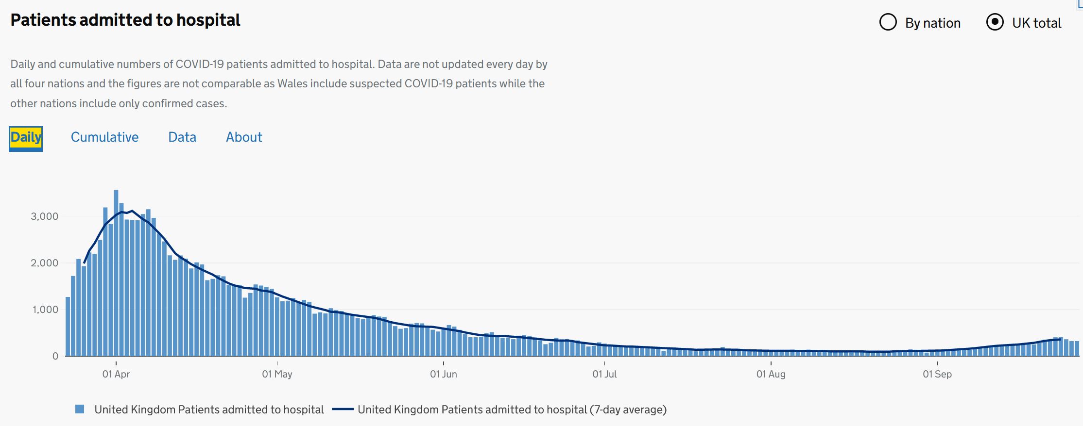
Many have responded by saying that it is daily COVID hospital admissions which is the key plot to focus on. It is certainly a better indicator of the COVID trend than just 'cases' and it is all plotted daily at https://coronavirus.data.gov.uk/. Here is today's plot shown on the site:

However, even if we ignore the major problem with the data for Wales (which artificially inflates the admissions data), there is still a problem in using this plot to monitor the progress of COVID. To see why, here is what the website says about the England data:

"data include people admitted to hospital who tested positive for COVID-19 in the 14 days prior to admission, and those who tested positive in hospital after admission. Inpatients diagnosed with COVID-19 after admission are reported as being admitted on the day prior to their diagnosis"

In other words, we have no idea how many of the 'COVID hospital admissions' were people actually admitted because of COVID. A person entering hospital for, say, cancer treatment who recently tested positive for COVID will be officially classified as a COVID case. The same is true of those entering hospital for any treatment who have not previously been tested positive for COVID but 'test positive' at some time during their stay. We have to therefore assume that - as in the public generally - a proportion of the 'COVID hospital admissions' are people who either a) don't have COVID; or b) are asymptomatic (or who will only ever have mild symptoms).

It also means that, as with 'COVID cases', much of the recent increase in 'COVID hospital admissions' may be explained by the general increase in number of people being tested. Unfortunately, we do not have the daily data for number of people being tested before and during UK hospital admissions. But it is not unreasonable to assume the number is roughly proportional to the total number of people being tested in the UK. So it makes sense to plot (using the data provided at https://coronavirus.data.gov.uk/) the daily hospital 'COVID admissions per 1000 people tested' in preference to simple the COVID admissions:

As data for number of people tested are only provided from 22 April, this plot does not cover the March period as in the plot above. However, you can see that the trend is similar except since 1 Sept, where the increase is more gradual. This suggest that, indeed some (but not all) of the recent increase is explained by the increase in testing.

Here is the same plot from 1 July:

And - before anybody suggests that it's "COVID deaths" not hospital admissions we should be looking at - everything I said above is also releant to those classified as COVID deaths.