Please go to https://www.normanfenton.com/post/the-curious-perfect-p-value-a-case-study-in-defamation-and-ignorance for an updated version of this article (there is also a problem with the graphics below).
1. The accusation
Kyle Sheldrick is making a name for himself as someone determined to expose those who he claims are guilty of spreading Covid ‘misinformation’. He has a particular obsession for going after people who promote real world studies of early effective Covid treatment. One such person is Paul Marik, a highly respected doctor with 30 years’ experience including pharmacology, anesthesiology, and critical care and many hundreds of highly cited peer-reviewed articles. Not content with trying to discredit the Covid work of people like Marik, on 22 March Sheldrick wrote a blog article in which he accused Marik and his co-authors of fraud relating to a 2017 study about vitamin C treatment for sepsis published in the CHEST Journal.

The basis for his potentially defamatory claims was that Marik’s study used data which Sheldrick said must have been fraudulent because the patients in the control group and treatment group were ‘too well matched’ for it to be by coincidence. The problem is that he used a statistical test to make this conclusion which he clearly did not understand, and which was in any case totally inappropriate for his (ill-defined) hypothesis of fraud.
Before analysing Sheldrick's claim it is important to note that Marik's study began as an observational study where the patient outcomes were good. In order to give the study more substance, the nurses went back in the same hospital patient data and pulled those that met the same criteria as those observed. This was a retrospective pairing and it was not meant to be random. But even ignoring this, Sheldrick's claim of fraud is wrong.
The problem is that, to make his conclusion, Sheldrick used a statistical test which he clearly did not understand, and which was in any case totally inappropriate for his (ill-defined) hypothesis of fraud.
Online researchers here and here have provided comprehensive explanations of the many reasons why Sheldrick’s argument is badly flawed. But missing so far has been an explanation of exactly what the statistic used by Sheldrick is and how it is computed. Once we show what it is, it becomes evident just how ludicrous the fraud claims are, even ignoring the fact that the control group patients were selected to be well matched.
2. Sheldrick's evidence
Sheldrick presents his ‘evidence’ in the form of this table:

The rows are the various attributes (personal or medical conditions) of the patients. There were 47 patients in the treatment group and 47 in the control group. The first (resp. second) column is the number of patients in the treatment (resp. control) group with the attribute, while the third (resp. fourth) column is the number of patients in the treatment (resp. control) group without the attribute. So columns 1 and 3 sum to 47 and columns 2 and 4 sum to 47.
Sheldrick’s hypothesis is that the control group and treatment group are too similarly matched in too many attributes for this to happen by chance (there are, for example, 6 of the 24 attributes where the numbers with the attribute are equal in both groups). He claims that the statistical evidence for this are the values in the last column. These values are the results of a particular statistical ‘significance’ test - the “p Value From Fisher Exact test” – applied to the first 4 column values. He claims that what you should be seeing here are values which average to 0.5 if there was no deliberate attempt to make the numbers in each group similar. The fact that so many numbers are equal to 1 and most of the others are above 0.5 is – according to Sheldrick - proof of fraud. But he is wrong, even if we ignore the various legitimate reasons (well covered in the article by Crawford) why there would inevitably be similarities.
3. So what is the "p Value From Fisher Exact test"
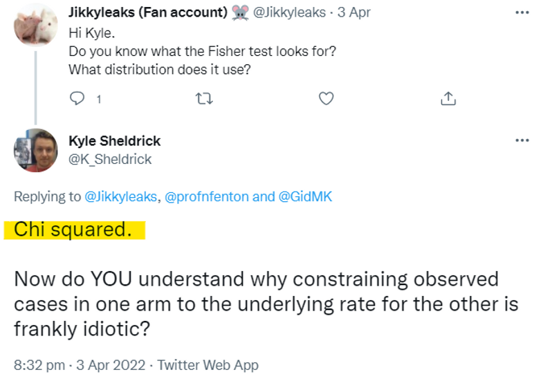
Those that know me know that, as a Bayesian, I regard any p-values and classical statistical tests of significance as arbitrary, overly complex and totally unnecessary (see Appendix below); many people who use them have no idea what they mean. But since this is what Sheldrick is using let's see exactly what the p value statistic in the last column of his table is. Sheldrick assumes that everybody knows what it is and how it is calculated. He does not provide a definition and, as this tweet shows, he does not know or understand it (it is NOT based on the chi squared distribution):
Instead, since he does not define or understand it, we can assume Sheldrick uses a pre-defined function (possibly in the R programming language or similar since this gives the same results to Sheldrick's) to compute it. In fact, there does not seem to be a ‘standard’ definition for this statistic and there are indeed online calculators like this that give completely different values to that of the function computed by R. For the general case it is quite a complex definition and calculation. However, when the total number of people in the control and treatment group are the same (which they are here, 47 in each) the definition and calculation of the test (as defined by the R function) is much simpler. So, I will stick with the definition and calculation for this simpler case because it allows us to show exactly how the numbers in Sheldrick’s final column are calculated and why they don't mean what Sheldrick thinks they mean.
The test is based on calculating the following probability:
Given that x+y patients out of 94 have a particular attribute, what is the probability that, if the 94 patients are randomly assigned to two groups of 47, exactly x patients in the first group have the attribute (this would mean exactly y patients in the second group have the attribute).
This probability is equal to the number of combinations of x in 47 multiplied by the number of combinations of y in 47 divided by the number of combinations of x+y in 94.
Mathematically, we write this as:

Formula 1 (it is also called the hypergeometric distribution)
So, for example, for the attribute malignancy, there were 5 in the control group and 7 in the treatment group. Applying Formula 1 with x=5 and y=7 we get:

So, the probability of getting exactly 5 in the control group and 7 in the treatment group (given that there were 12 in total) is 0.202. But we need to do some more calculations before getting the 'p-value exact Fisher test' value as defined in the function used by Sheldrick.
First, we note that the difference between the numbers (5 and 7) is 2. That might be considered quite a small difference. As there are 12 in total with malignancy, we calculate the combinations with a difference greater than observed: 12 (12 in control group and 0 in treatment, or 0 in control and 12 in treatment), 10 (11 and 1, or 1 and 11), 8 (10 and 2, or 2 and 10), 6 (9 and 3, or 3 and 9), 4 (8 and 4, or 4 and 8). In fact, the ONLY way we would have observed a difference of less than the 2 we observed is if we had observed 6 in each. The probability of observing 6 in each is, according to Equation(1), equal to 0.2414.
So, the probability of observing at least as big a difference to what we observed is simply 1 minus 0.2414 which is 0.7586 which is the number in the final column.
So, (in the case where the group sizes are equal), the statistic is defined as the probability of observing at least as big a difference as the one actually observed.
To further illustrate this from first principles, look at the diabetes attribute. Here we have 16 and 20 respectively from the treatment and control groups. That is a difference of 4. The only way we could have observed a smaller difference is with the pairings:
- (17, 19) which has a probability 0.15371 (difference 2)
- (19, 17) which has a probability 0.15371 (difference 2)
- (18, 18) which has a probability 0.167844 (difference 0)
So, the probability of observing a smaller difference is the sum of these three probabilities which is 0.474264. And, therefore, the probability of observing at least as big a difference as the one actually observed is 1 minus 0.474264, which is 0.524736 which is the number in the final column.
For attribute drug addiction the number observed is 5 in each, so the difference is 0. The probability of observing numbers with a lower difference than that is 0 because there are no such possibilities. So, the probability of observing a difference at least as large as what was observed is 1, which is the number in the final column.
But we must also always get 1 in the final column when the difference observed is 1 because this means there are an odd number of people with the attribute in total, and it is impossible therefore to observe a difference of 0. That means the probability of observing at least as many as 1 is 1. Take, for example, no comorbidity with 2 in the control group and 1 in the treatment group. The only possible combinations we could have observed here are
- (0, 3) which has probability 0.121
- (3, 0) which has probability 0.121
- (1, 2) which has probability 0.379
- (2, 1) which has probability 0.379 (this was what was observed)
None of these has a difference less than 1 and you can see that these 4 probabilities sum to 1.
But this no comorbidity example reveals how inappropriate Sheldrick’s use of the statistic is. Sheldrick claims that getting a 1 for the statistic is an indication that this was an unusually low difference and therefore is unlikely to have happened by chance. But the actual probability of observing a difference of exactly 1 in this case is equal to the probability of observing (1,2) plus the probability of observing (2,1). That’s a probability of 0.758. In other words, contrary to what Sheldrick believes, it would actually have been far more unusual to have observed the other possibility (a difference of 3). If we had observed a difference of 3 then the statistic in the final column would have been 0.242 rather than 1.
Let’s look at some other examples where the p-value is 1 and see how 'unusual' the observations really are:
- COPD has pairing (8,7), a difference of 1. The probability of observing this combination is 0.213 – the same as the probability of observing (7,8). So the probability of observing this difference of 1 is 0.426. That is not at all unusual.
- CRF has pairing (7,8), a difference of 1. The calculation here is the same as COPD - the probability of observing a difference of 1, when the total with the attribute is 15, is 0.426.
- Urosepsis has pairing (11,10), a difference of 1. The probability of observing a difference of 1 when the total with the atribute is 21 is 0.38. Again, not unusual.
- ‘drug addiction’ has pairing (5,5), a difference of 0. The probability of observing this is 0.26, which you can hardly consider as ‘highly unusual’.
4. So how may of the pairings really are 'unusually similar'?
In Table 2 we compare the p value with the (much more meaningful) probability of observing the difference - or smaller - in the particular pairing observed (that was shown in Table 1)

The average of the probabilities of observing the difference observed or less is close to 0.5.
The most ‘unusually similar’ pairing is the (22,22) pairing for vasopressors. But even this has a probability of 0.1636.
Only two attributes (vasopressors and positive blood cultures marked in yellow) have an 'unusually similar' pairing if we assume this is defined as one for which the probability of getting the observed difference (or smaller) by chance is less than 0.2.
Perhaps the threshold of 0.2 is too low to conside a pairing to be 'unusually similar'. What if we raise the threshld to 0.3? Even then only four other attributes (those highlighted in orange in Table 2) are added to the set of 'unusually similar' pairings.
5. So what does the number of 'unusually similar pairings' really tells us about the probability of fraud'?
'Well, we can approximate the probability using some basic maths. The average probability of the 'unusually similar' pairings is about 0.2. So let's assume that the probability of getting an 'unusually similar' pairing is 0.2. Now, if there were only 6 attributes in total and all 6 had 'unusually similar' pairings, then the probability that this would happen by chance is 0.2 to the power of 6 which is 0.000064 (0.00064%); that is 1 in 15,625. That still doesn't tell us what the probability of fraud is, but it does tell us how incredibly unlikely it is that such an observation would happen by chance. If there were, say, 12 attributes in total then, by the Binomial theorem, the probability of observing at least 6 'unusually similar' pairings would be 0.0194 (1.94%). But with 24 attributes in total, the probability of observing at least 6 unusually similar pairings is 0.3441 (34.41%). In other words there's a greater than 1 in 3 chance of getting such an observation by chance.
To compute an actual probability of fraud given the evidence we need a Bayesian analysis and some other assumptions. Such an analysis is provided in the Appendix. In this we explicitly assume that, under the 'no fraud' hypothesis the probability of an unusual pairing is a uniform distribution between 0.1 and 0.3. Under the 'fraud' hypothesis we assume the probability of an unusual similar pairing is a uniform distribution between 0.3 and 0.6 (anything higher would be 'too obvious'). With these assumptions, under the 'no fraud' hypothesis the probability of observing at least 6 unusually similar pairings is 36.3% (whereas under the fraud hypothesis it is 98.1%). If we assume, as a prior, that the fraud and no fraud hypotheses are equally likely, then for the observed 6 unusually similar pairings, the posterior probability of fraud actually decreases to 26%. In other words, the evidence does not support the fraud hypothesis.
6. The ramifications and what's next
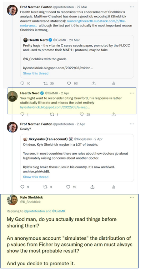
Sheldrick and his friends on twitter not only savaged the reputation of Paul Marik on the basis of their flawed understanding of statistics, they also ridiculed my credentials as a mathematician for daring to like/retweet the articles by Mathew Crawford and others who highlighted Sheldrick's statistical illiteracy:


It may be that Sheldrick’s intentions are honourable but that he has been egged on by other more senior figures determined to bring down all those promoting early Covid treatments. He could redeem himself by 1) apologising for his attack on Marik and 2) exposing those senior figures who have put him into this compromising position.
7. Update
Sheldrick has, in a seemingly endless stream of tweets, tried to discredit this article. The core of his complaint is this:
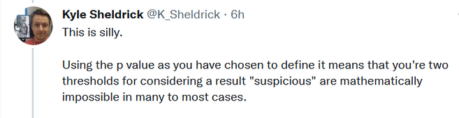
But in his own reponse to Matt Crawford's critique of his letter he includes a section "Part 2: How I would criticise my original post if I wanted to try and tear it down" which essentially acknowledges that is is indeed mathematically impossible to get very low probabilities of observing smaller differences in most cases. So, if anything he seems to agree with me there, and it's not clear then what his argument is. Sheldrick never provides definitions nor any details of exactly what his hypotheses are in his original claim of fraud (i.e. the assumptions which presumably don't apply to those in his 'Part 2'). His claim might make sense based on the following erroneous assumption: that, for any given attribute, you can assume that the number of people in a group of 47 with the attribute is any number between 0 and 47. So even if, (as in the example of the attribute 'no comorbidity') only 3 people out of the 94 had this attribute then perhaps he is assuming that we should be just as likely to observe 47 out of 47 with that attribute as 0 out of 47. In fact, the assumption I clearly stated was that the total you would see in each group is bounded by the total number of people in the two groups who have the attribute. So, in the 'no comorbidity' example, the ONLY possible way these could have been assigned to the two groups is:
- 3 in one and 0 in the other (which occurs with probability 0.242); or
- 2 in one in 1 in the other (which occurs with probability 0.758)
Since a (2,1) pairing was observed (i.e. a with a difference of 1 between them) then it really is impossible to observe a difference less than what was observed, and so the probability of getting a matching where the difference is less than or equal to the one observed is 0.758.
Now - as was already explained in the Appendix below - it is reasonable to argue that the total observed with the attribute (3 out of 94) does NOT mean that it is impossible to observe a higher number than 3 out of 47 in a new group. But to use that argument we would need to use the observed proportion (e.g. by Bayes) to estimate the 'true' patient population proportion for this attribute. That would indeed change the calculations (but not by very much). But that is not what Sheldrick does.
Update: Here is a video covering the main issues:
8. A hypothetical example that shows just how ludicrous Sheldrick's accusations are
Imagine the following:
In a large British senior school all first years (these are 11-12 years olds unless they missed a year or more) take an English test after 2 weeks. Those who fail get retested 2 weeks later.
In a trial, 47 of those who fail are given some short one-to-one tutoring before the next test and the results are very promising, as 42 of them pass the next test. To determine how effective this short tutoring session is the results (from second test) of a selection of 47 students who did NOT get the tutoring are reviewed. Only 10 of them passed the second test. These results for short tutoring are considered so good that the study is published and short tutoring is subsequently recommended to all students who fail the first test.
However, 5 years later an anti-tutoring activist declares the study was fraudulent because there was an impossibly close matching between the tutored group and the control group -which could not have happened randomly, as evidenced by the large number of Fisher exact p statistic values equal to 1:

Note how the type of criteria, their underlying population rates, and inevitable dependencies and correlations between them, mean that it would be remarkable if you did not see a lot of p-values equal, or close, to 1.
9. Sheldrick's behaviour
As pointed out by an online researcher this is the kind of online hate posted by Sheldrick (this time against an esteemed cardiologist) that not only contravenes good medical practice guidelines, but also shows that he doesn't understand the difference between "heart attack" and "sudden cardiac death".

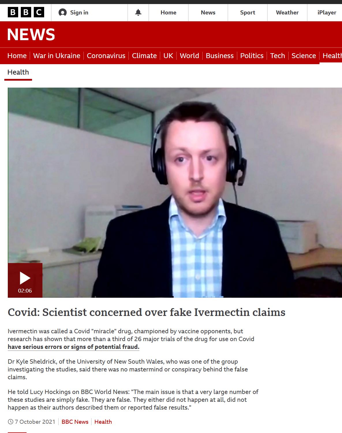
There is plenty more on Sheldrick's dubious associations and funding here. So how comes the BBC decided that this guy was a suitable 'scientist' to interview?
Appendix: Bayesian analysis
If you want to test a hypothesis then you want to be able to conclude something about the probability that the hypothesis is true based on the evidence you find; and for that you need a Bayesian approach which avoids any dependency on p-values.
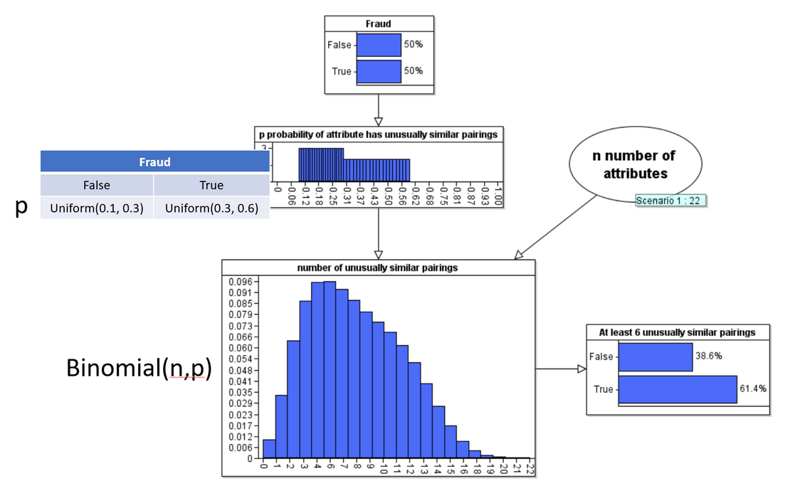
In the following Bayesian network model we assume the 'Fraud hypothesis is either true or false'. Here we assume a 50-50 prior. Our assumption about what 'fraud' actually means is encoded into the definition of the conditional probability function for the node p ('probability attribute has unusually similar pairing'). Here we explicitly assume that, if Fraud is false then p is a uniform distribution between 0.1 and 0.3 and if Fraud is true then p is a uniform distribution between 0.3 and 0.6 (we can easily run the analysis with different assumptions but all of these assumptions are quite favourable to the fraud hypothesis).
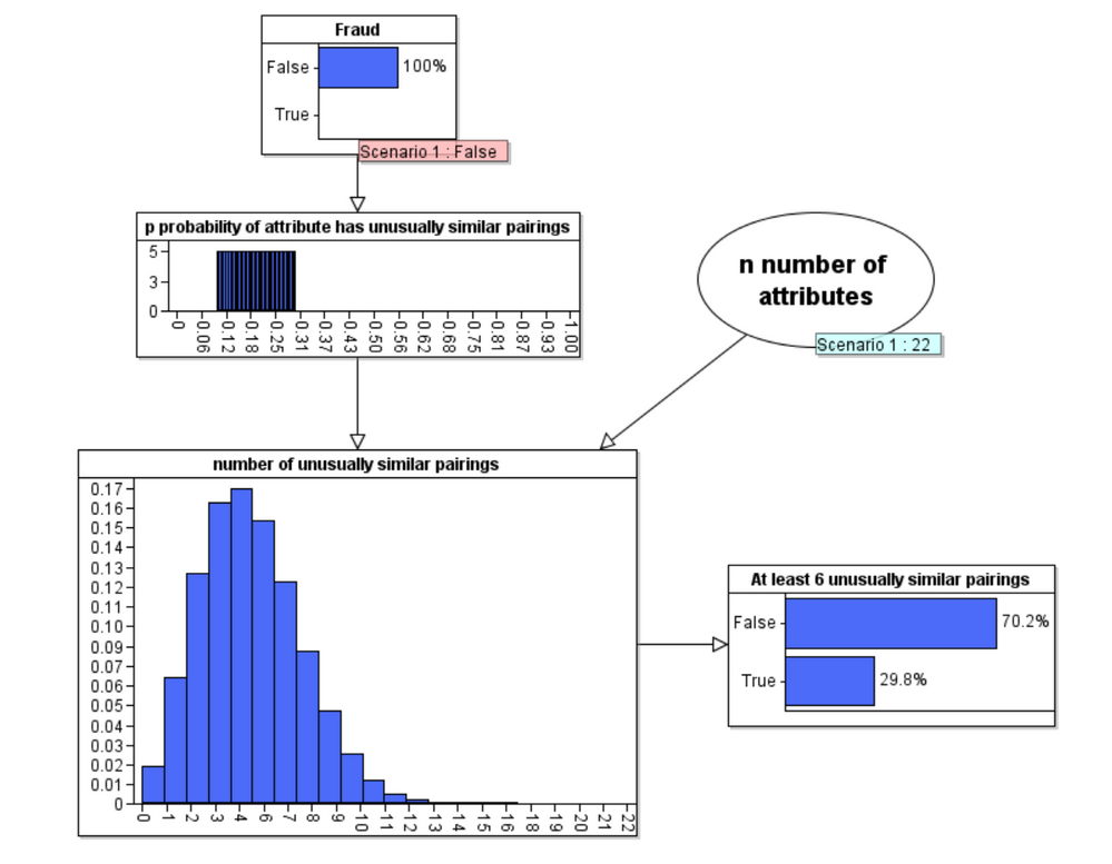
When we run the model under the Fraud = false hypothesis we get the following updated probabilities:
But, of course the real power of Bayes is in its backward inference that enables us to compute the revised posterior probability of Fraud when we observe 6 unusually similar pairings:
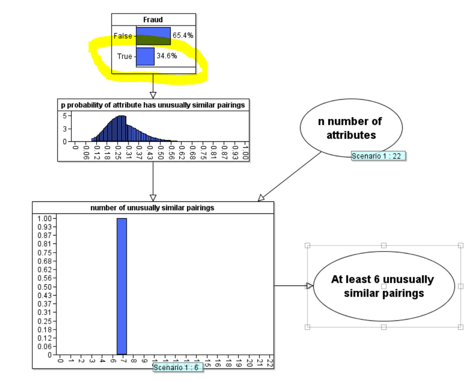
As you can see the posterior probability that Fraud is true has decreased to 34.6%. Contrary to what Sheldrick assumes the evidence does not support his accusation of fraud.
(Note: A really comprehensive Bayesian analysis would do something much cleverer than assume the chosen uniform distributions in the node p. Also, for each attribute we would take account of any prior knowledge about the incidence rate for the attribute and use the number of observed cases of the attribute in the 94 patients to produce an updated probability of observing the attribute in a patient. We would then use this information to determine the probability of observing the particular observed pairing for that attribute by chance. The Bayesian estimate for fraud is also ceiling on the likely true value of fraudulent data due to the likelihood of a fat tailed distribution of attributes of sepsis patients during different time intervals and correlations between various attributes).